1 Introduction
The Continuous Wavelet Transform (CWT) of a signal  in the
  basis is defined as
 |
(1) |
It can be interpreted as the correlation of the input signal with a mirrored
version of  , which is rescaled by
  . For
a 1-D input, the result is a 2-D time-frequency description of the signal.
The scale is proportionally inverse to the frequency studied, and
. For
a 1-D input, the result is a 2-D time-frequency description of the signal.
The scale is proportionally inverse to the frequency studied, and  represents the time localization at which we analyze the signal. The bigger
the scale
represents the time localization at which we analyze the signal. The bigger
the scale  the wider the analyzing function , and hence
the smaller the corresponding frequency. The big advantage over FT is that the
frequency description is time localized, and hence evolves in time.
the wider the analyzing function , and hence
the smaller the corresponding frequency. The big advantage over FT is that the
frequency description is time localized, and hence evolves in time.
Fast implementations of the Wavelet Transform take into account multiresolution
properties of wavelet functions to compute the CWT at dyadic scales  and time-shifts
 . Using Mallat's algorithm or derivatives,
they get an overall
. Using Mallat's algorithm or derivatives,
they get an overall  complexity. Other techniques compute the Wavelet
Transform at dyadic scales and at linear time-points, or, by using
complexity. Other techniques compute the Wavelet
Transform at dyadic scales and at linear time-points, or, by using  mother wavelets closely dilated, at M-adic scales. Other methods compute the
CWT at integer scales (
mother wavelets closely dilated, at M-adic scales. Other methods compute the
CWT at integer scales ( ).
).
We present a new method, using expansion of both the input signal and the mother
wavelet in B-Spline basis, that computes the CWT at any real scale, allowing
to zoom in the frequency domain. This method also gets rid of recursivity scheme
present in the previous methods, and fits well to parallel implementation.
2 Review of B-spline properties
Basic Definitions
The B-spline (``B'' standing for ``Basic'')  of degree
 is defined as
 |
(2) |
The B-spline  of degree
  is defined as the
  convolution of with itself :
 |
(3) |
Now, we enumerate a series of definitions that are necessary in our formalism
:
Continuous Operators :
- Derivative :
 |
(4) |
- Integral :
 |
(5) |
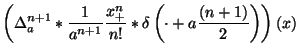
- One-sided power function :
 |
(6) |
which is equivalent to the (n+1)-fold integral operator since :
 |
(7) |
Discrete Operators
- Finite differences :
 |
(8) |
- Inverse finite differences operator :
Using these definitions, a B-spline of degree can
be written as:
 |
(10) |
Intuitively, this means that the convolution with a B-spline of degree
is equivalent to shift the signal by  , to integrate it
times, and to apply
, to integrate it
times, and to apply
 times a finite differences operator
to the result of the integration.
times a finite differences operator
to the result of the integration.
Using the exchange rules for the one-sided power function and for the shift
with the rescaling operator given in , and noting that the rescaled finite differences
operator
 can be expressed as
 |
(11) |
while a B-spline of order and rescaled by a scale writes :
Finally, we define the mixted convolution of a continuous signal  with a discrete one
  with intersample distance equals to
as:
with intersample distance equals to
as:
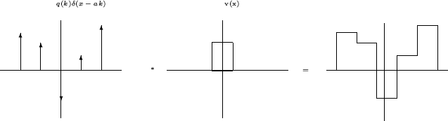
Figure 1:
Graphical Interpretation of the mixted convolution : weighted sum of shifted
versions of the function v(x)
 |
B-spline Interpolation
Splines are one of the most famous family of interpolators : given a sampled
signal, know for example at integer points, one easily interpolates it at any
real point, conserving essential properties such as smoothness. Unser describes
the power and the efficiency of B-spline interpolation, which allows to get
rid of all the matrician inversion calculated in conventional spline-interpolation.
Given an input signal, its B-spline description is easily obtained via simple
digital filtering, using IIR filters with fast recursive implementations.
B-spline Wavelets
Among all existing wavelets, that verify the admissibility conditions, B-spline
wavelets have the advantage of being explicitly known, and of not depending
on recursive definitions. The famous Haar-wavelet is just the sum of two B-splines
of degree 0. Other wavelets, such as the first derivative of a Gaussian () or
the second derivative (Mexican wavelet) can be closely approximated by B-splines
of higher degrees . The corresponding approximation errors of a Gaussian are
negligible at small scales, and tend to when the B-spline degree grows.
This expression (14) of wavelets into B-spline
basis (through either orthogonal or oblique projections) allows to compute the
inherent convolution products of the CWT in B-spline basis efficiently, taking
advantage of properties such as compact support (convolutions are computed on
finite -and small- number of points).
According to all these considerations, we may now suppose that the mother wavelet
is expressed in a B-spline basis of order  :
:
 |
(14) |
3 Real CWT Computation in B-spline basis
General case
Using (10), and thanks to commutation properties
of the convolution operator, the CWT
 becomes :
 |
(15) |
This shows that the wavelet transform can be seen, for each weight  ,
as the application of a modified finite differences operator to the
,
as the application of a modified finite differences operator to the
 -th
integral of a shifted version of the analyzed function .
-th
integral of a shifted version of the analyzed function .
Expanding the modified finite differences operator
 in the previous results yields:
(with
 ), which is
a particular case (finite sum) of a mixted convolution defined in (13).
), which is
a particular case (finite sum) of a mixted convolution defined in (13).
B-spline description of the analyzed function
If we consider that our input signal  belongs to a B-spline space
of degree
belongs to a B-spline space
of degree  ,
,
where the interpolation coefficients  were determined by
 ,
with
,
with
 representing the discrete samples of
the B-spline of degree (B-spline kernel), and
representing the discrete samples of
the B-spline of degree (B-spline kernel), and  representing sampled at integer points.
We can rewrite as :
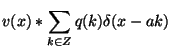
![\begin{displaymath}
v(x)=A(a)c_{f}*\left[ \sum ^{K}_{k=-K}d_{k}D^{-(n_{1}+1)}\be...
...}}\left( x+a\left( \frac{n_{1}+1}{2}-k\right) \right) \right]
\end{displaymath}](img60.gif) |
(20) |
But :
thus :
with
 and
and
 .
.
Going back to the mixted-convolution expression of the CWT, the previous relation
yields :
where
 .
.
Finally, we use the compact support property of B-splines :
vanishes outside
 . Consequently,
the only non-null coefficients of
. Consequently,
the only non-null coefficients of
 are given by:
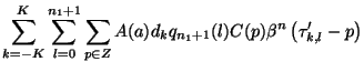
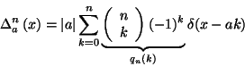
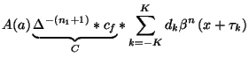
By calling
 ,
we obtain the final expression of the CWT :
,
we obtain the final expression of the CWT :
 |
(26) |
Comments
According to (23),(25) and (26),
the weights
 are equal to :
 |
(27) |
where  is an integer value between and
The 'big' number of dimensions (3) of this filter can be explained easily. The
index ' 'corresponds to the decomposition of the initial wavelet into
 weighted and rescaled B-splines ;
  corresponds to the decomposition
of each of these rescaled B-splines. Finally,
corresponds to the decomposition
of each of these rescaled B-splines. Finally,  corresponds to the
convolution of B-splines from the signal decomposition with the ones from the
rescaled wavelet description.
corresponds to the
convolution of B-splines from the signal decomposition with the ones from the
rescaled wavelet description.
Usually, corresponds to the time locations of the sampled signals and
takes thus integer values. The shift by in  cancels
out with the corresponding shift of
cancels
out with the corresponding shift of  That means that the values
of
remain the same for , and
That means that the values
of
remain the same for , and  fixed, whatever . This reduces considerably the number of weights since
only
fixed, whatever . This reduces considerably the number of weights since
only
 need to be computed.
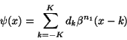
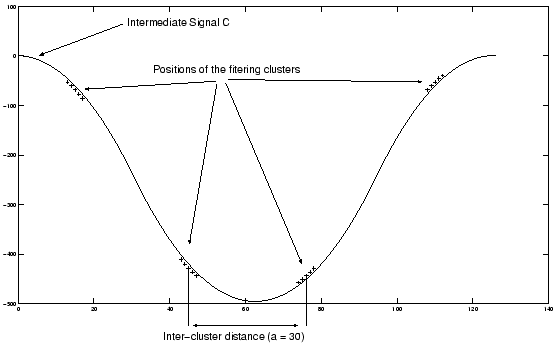
It is also interesting to study the localization of the weights. We first freeze
the index . One can observe that, for fixed, the weights are
modulated values of B-spline, uniformly distributed with a step of 1 (we call
it a 'convolution cluster'). Then, when we increment of decrement ,
values of the B-spline may or may not be equal, depending on the value of ,
but the central value and the lower bound  are
simply translated by . Hence for fixed, the CWT consists in
filtering
are
simply translated by . Hence for fixed, the CWT consists in
filtering  with
with  'clusters' of length
  each
cluster being separated from its neighbors by a distance . This can
be seen as a kind of modified 'a trous' filter, as shown in figure 2.
Moreover, when is incremented or decremented, the whole set of clusters
corresponding to a -index is also shifted by since
and play the same role in (27).
each
cluster being separated from its neighbors by a distance . This can
be seen as a kind of modified 'a trous' filter, as shown in figure 2.
Moreover, when is incremented or decremented, the whole set of clusters
corresponding to a -index is also shifted by since
and play the same role in (27).
Figure 2:
Localization of the weights w(a,k,l,m) for k fixed, a=30, n1=3, n2=0
|
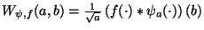
Fast Implementation
We have developed a fast algorithm for the computation of the CWT at any real
scale and any integer time-localization by using equation
(26) and the study of the filter 
As initialization step, we compute the values of the weights  .
This coefficients may be stored for pre-calculated cases (pre-defined wavelets
and their B-spline expansion coefficients and expansion
degree , interpolation degree and pre-defined values
of the scales ).
.
This coefficients may be stored for pre-calculated cases (pre-defined wavelets
and their B-spline expansion coefficients and expansion
degree , interpolation degree and pre-defined values
of the scales ).
In a first step, the B-spline expansion coefficients of the sampled
signal are calculated, and the finite differences operator
 is applied
times. The intermediate
result does not depend on the scale
is applied
times. The intermediate
result does not depend on the scale 
The second step, repeated for all the values of , consists in filtering
with the stored values of  . The dependence with regards to
only concerns the values of chosen and the inter-cluster distance
for the filtering, but the complexity per point is fixed by the values of
. The dependence with regards to
only concerns the values of chosen and the inter-cluster distance
for the filtering, but the complexity per point is fixed by the values of  and . It has to be noticed that the independence between
scales allows straightforward parallel implementations. The algorithm is described
in figure 3.
and . It has to be noticed that the independence between
scales allows straightforward parallel implementations. The algorithm is described
in figure 3.
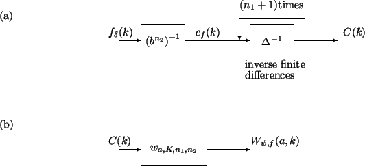
Figure 3:
Fast implementation of the fast CWT.
(a) : Initialization, (b) :
scale dependent step
 |
4 Complex CWT (Gabor-Like CWT, CCWT)
The Continuous Wavelet Transform we used so far supposed that the mother wavelet
was a real function. Such a transform can be considered as a correlator,
where the correlation pattern is rescaled by This method
is very efficient for edge detection, singularities characterization (Hölder
exponent), ... , but does not really give us a time-frequency description of
the signal (in the sense of a Fourier Transform indicating which sinusoid frequencies
are present in the signal). An efficient method for the characterization of
the period of evolving signals is the Complex Continuous Wavelet Transform (Gabor-Like
CWT). This CCWT is based on a complex wavelet, namely a complex exponential
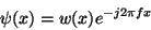
of frequency windowed by a Gaussian :
 |
(28) |
This wavelet transform is relatively similar to the Short Time Fourier Transform,
but since the gaussian window is a function of  , it will grow in width
for large scale and hence keep a constant ratio between analyzing period and
concerned frequency, keeping a constant precision over scales. Unser
() described a fast implementation of this transform using B-splines in order
to approximate the gaussian function. The key idea is that the central B-spline
converges to a Gaussian uniformly when tends to infinity.
For
, it will grow in width
for large scale and hence keep a constant ratio between analyzing period and
concerned frequency, keeping a constant precision over scales. Unser
() described a fast implementation of this transform using B-splines in order
to approximate the gaussian function. The key idea is that the central B-spline
converges to a Gaussian uniformly when tends to infinity.
For  , the variance product is already within
  of the limit
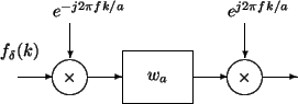
specified by the uncertainty principle. In order to compute the Complex CWT,
Unser proposes a modulation approach : the input signal is first modulated by
a complex exponential
of the limit
specified by the uncertainty principle. In order to compute the Complex CWT,
Unser proposes a modulation approach : the input signal is first modulated by
a complex exponential
 , then filtered through the window
 at scale , and finally demodulated by an other exponential
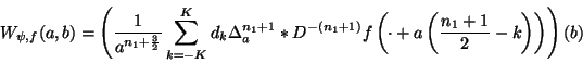
 , as shown in figure 4. At a scale the CCWT
is thus equivalent to the correlation of the input signal with a windowed complex
exponential whose frequency is
, as shown in figure 4. At a scale the CCWT
is thus equivalent to the correlation of the input signal with a windowed complex
exponential whose frequency is  that means, for an initial
frequency of
that means, for an initial
frequency of  (common case), the scale simply corresponds
to the period. Usually, the modulus of the CCWT is displayed in a scalogram,
a 2D-plot where the x-axis is the time , and the y-axis corresponds
to (Figure 4).
(common case), the scale simply corresponds
to the period. Usually, the modulus of the CCWT is displayed in a scalogram,
a 2D-plot where the x-axis is the time , and the y-axis corresponds
to (Figure 4).
Figure 4:
Computation of the Complex CWT by modulation, gaussian-windowing and demodulation
 |
The link with our method is rather obvious. Excepted the pre- and post-modulations
by complex exponentials, we may consider the filtering window as a wavelet
described in a B-spline basis, where the coefficients of (14)
are one for  and zero otherwise. The Gaussian is approximated by a
B-spline of degree
and zero otherwise. The Gaussian is approximated by a
B-spline of degree  So we used the same algorithm, but replaced
the real cwt method used at integer scales by ours in order to be able to compute
it at any scale.
So we used the same algorithm, but replaced
the real cwt method used at integer scales by ours in order to be able to compute
it at any scale.


![$\displaystyle A(a)c_{f}*\left[ \sum ^{K}_{k=-K}d_{k}\Delta ^{-(n_{1}+1)}*\beta ...
..._{2}+1\right) }\left( x+(a-1)\left( \frac{n_{1}+1}{2}\right) -ak\right) \right]$](img64.gif)
![$\displaystyle A(a)C*\left[ \sum ^{K}_{k=-K}d_{k}\beta ^{n}\left( x+\tau _{k}\right) \right] *\sum ^{n_{1}+1}_{l=0}q_{n_{1}+1}(l)\delta (b-al)$](img68.gif)