The goal of this session is to implement several 2D deconvolution algorithms. The implementation will be done entirely in the Fourier domain.
1. Coding the Fourier operations
1.1 FourierSpace object
To make the task easier, a FourierSpace class is provided (class FourierSpace). This class contains:
| Public Members | Description | Example |
| double real[][] | double array containing the real coefficients of the Fourier transformation | G.real[fx][fy] = 10.0; |
| double imag[][] | double array containing the imaginary coefficients of the Fourier transformation | G.imag[fx][fy] = 10.0; |
| int nx | Size in X of the Fourier space | int sizex = G.nx; |
| int ny | Size in Y of the Fourier space | int sizey = G.ny; |
| Constructors | Description | Example |
| FourierSpace(nx, ny) | Creates an empty Fourier space of size [nx,ny] corresponding to [0..2π,0..2π] | FourierSpace G = new FourierSpace(nx, ny); |
| FourierSpace(image) | Creates a Fourier space containing the Fourier transformation of a ImageAcces object | FourierSpace G = new FourierSpace(image); |
| Public Methods | Description | Example |
| void transform(image) | Fill the Fourier space with the transform of an ImageAccess object | G.transform(image); |
| ImageAccess inverse() | returns an image that is the inverse Fourier transform. | ImageAccess g = G.inverse(); |
| void fillSym(double[][] function) | fill the whole [0..2π][0..2π] Fourier space based on a function defined in [0..π][0..π] | G.fillSym(function) |
| void showModulus(String title) | Shows the modulus of a FourierSpace object | G.showModule("G"); |
1.2. Implemention of operations for the FourierSpace objects
Get inspiration from the routine add() that adds two Fourier Space objects (complex coefficients) to write the divide() and the 2 multiply() routines. To avoid instabilities, never divide by a modulus of the denominator lower than ε (less than ε, e.g. 1E-9).
Check your operators using the plugin TestFourierMultiply and TestFourierDivide that multiples or divides the Fourier transform of an image (forest.tif) by the identity filter.
1.3 Implementing basic filters in the frequency domain
Write the following filters in the frequency domain.
| Java routine name | Freq. response (ω is the radial frequency: ω2 = ωx2 + ωy2 ) | |
| identityFourier(nx, ny) |  |
The code is provided as example |
| gaussianFourier(sigma, nx, ny) |  |
To be written for question 2 σ is the standard deviation of the gaussian |
| laplacianFourier(nx, ny) |  |
To be written for question 2.2 |
| otf(d, nx, ny) Model of a symmetric Optical Transfer Function that simulates defocussing of a microscope lens. |
K = 275 . 10-6, σ = sqrt(3), zi = 2000 μm, d is the out-of-focus distance To be coded for question 3 d is given in μm in the dialog box and already converted to m for the routine otf() |
|
It is sufficient to compute the symmetric filter function F(ω) = F(ωx,ωy) between [0..π ][0..π]. The Java method fillSym() will fill the Fourier space using hermitian symmetry. Be careful: F(ω) should be explicitly defined for ωx=π and ωy=π. Thus, these routines should create a 2D array function[nx/2+1][ny/2+1]:
Observe the impulse response and the frequency response of your filters using the plugin Display Filter.
Convolve the image cat.tif with the following filter: Gaussian (σ=6), Laplacian and OTF (d=6 μm) using the plugin Convolve. Insert the result images in the report.doc
2. Deconvolution based on a gaussian model
For this question, we assume that an image is blurred with a 2D gaussian filter Hσ(ω) defined in the Fourier domain. The goal is to evaluate the performance of four deconvolution algorithms on noisy images when the model is not perfectly known. The input image is an ImageAccess object g(x,y) and G(ω) is the Fourier transform of g.
2.1 Inverse filtering restoration
Implement the inverse filter deconvolveInverseFilter().
This routine has to return f(x,y) which is the inverse Fourier transform of F(ω)
2.2 Regularized least-square restoration
Implement the inverse filter deconvolveRegularized().
This routine has to return f(x,y) which is the inverse Fourier transform of F(ω):

L(ω) is the laplacian function. Use the stabilized division (up to the limit ε) to make the division in the complex Fourier domain.
2.3 Landweber algorithm
Implement the Landweber iterative filter deconvolveLandweber(g, H,γ,n) that performs an iterative least-square restoration.
This routine has to return f(x,y) the inverse Fourier transform of F(k)(ω) where k is a predefined number of iterations.
2.4 Landweber algorithm with the positivity constraint
An improvement of the previous algorithm is to limit the dynamic range of the signal. Implement the iterative constraint filter deconvolveLandweberPositivity(g, H,γ,n). The routine has to return f(x,y) following the same recursive equations as 2.3. At each step of the iterative loop, add a positivity constraint that limits the intensity to positive values in the spatial domain.
2.5 Comparison of the algorithms
Compare the algorithms in terms of computation time and quality (SNR). In particular, we want to check their robustness to noise and to modelling errors.
Create three degraded images with a gaussian blurring (σ=2.0) and increasing levels of noise:
Compare the robustness of the 4 algorithms and insert the results in the file report.doc.
The settings of the algorithms are indicated in the report.doc. Measure the SNR: choose the reference image moon.tif and press "Deconvolve+SNR" in the plugin Deconvolve
2.6 Settings of the iterative algorithms
Iterative algorithms often give better results when they are stopped after a suitable number of iterations. The main difficulty is to find the parameters of the loop: the relaxation parameter γ and the number of iteration n. Try to find experimentally γ and n giving the highest SNR for Landweber algorithm restoration of the blurred and noisy image: moon_degraded.tif (gaussian σ=1.5, noise=4). We provide a way to visualize the steps of the iteration: choose "Teacher: Landweber", select "Display iterations step", choose the reference image moon_small.tif and press "Deconvolve + SNR".
3. Application: deconvolution of microscope images
A microscopist has acquired a blurred image of cell nuclei on a microscope. We assume that the optical transfer function of the microscope is given by otf(d,nx,ny) in question 1. Try to restore the blurred image cap_cells.tif to make it possible to distinguish the fluorescent spots in the membrane of the nucleus. Choose OTF model (d=6 μm), and select the best algorithm and parameters. The results are evaluated visually. Report your settings and insert the resulting image in report.doc.
| Blur image | Example of result |
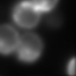 |  |