1. Introduction
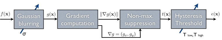
We propose to implement an efficient version of the Canny-Deriche edge detector. The algorithm will be implemented step by step following this diagram.
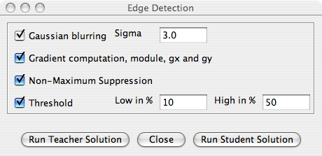
To call the implemented Edge Detection methods in ImageJ, use the plugin Edge Detection and select the desired operations through the dialog box. This plugin shows only the output of the last operation. Use the test.tif image to check the different steps of this algorithm.
|
|
| ||||||||||||
2. Gaussian blurring
We choose the Gaussian filter as our smoothing operator. It is implemented efficiently through a cascade of N symmetric exponential filters. In practice we choose N=3. The value of the standard deviation σ (equivalent window size) is entered through the dialog box.
2.1 Determination of the poles
The equivalent variance σ2 of a cascade of filters is the sum of the variances of the individual operators; here, σ2= 2Na/(1-a)2. Find the relation between σ, N and the pole values to be used in Section 2.2.
2.2 Implementation of a 2D Gaussian filter
Write the routine blurring(), which implements the Gaussian filter in a separable manner,
in the file Code.java. We provide a method named:
double[] out = Convolver.convolveIIR(double input[], doubles poles[]);
that performs the symmetrical IIR filtering of a 1D signal input[]
with a filter defined by its poles poles[].
Replace a=0.5 in the code by the correct pole value (a<1).
If you do not succeed, call TeacherCode.blurring().
3. Gradient computation
3.1 Implementation of gradient filters
|
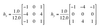
Write the code for filtering an image with hx and hy in the method gradient(). The output of the routine should be an array of 3 images ImageAccess grad[3]:
|
|
We recommend a separable implementation which is faster, but you may also use a non-separable one which is easy to code if you wish. In the first case, don't forget to implement the mirror boundary conditions in the 1D filtering explicitly.
If you do not succeed, call TeacherCode.gradient().
4. Non-Maximum Suppression
 4.1 Determine the positions A1 and A2
For a point A = (xA, yA) in the image, you have to compute the position of the points:
Avoid using trigonometric functions because they are not efficient.
4.2 Implementation
Write code that implements non-maximum suppression by using the following algorithm: The magnitude value G(A) is kept only if it is greater or equal to G(A1) and G(A2) and if G(A) is not equal to 0, otherwise it is suppressed; i.e., set to 0.
To compute G(A1) and G(A2) use an interpolation routine that returns a computed image value at any spatial location (xa, ya)—not necessarily integer. This method of ImageAccess can be invoked thus:
double ga, xa, ya;
ga = image.getInterpolatedPixel(xa, ya);
If you cannot answer this question, call Teacher.suppressNonMaximum().
5. Hysteresis Threshold
The contour segments above a Thigh (high threshold) are grown in a way to include all connected points greater than Tlow (low threshold). The values of the two thesholds are entered through the dialog box as percentage of the maximum of the gradient. The routine is provided.
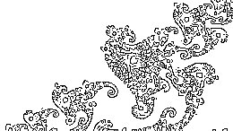
Apply the edge detector to obtain different levels of detail (as shown below) in the edges of the "mandelbrot.tif" image by adjusting the parameters σ, Thigh and Tlow. Save the parameters and the output images and insert them in the report.doc.
 |
 |
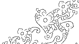 |
| Original image | Expected result: Details | Expected result: Global |
6. Application: water level measurement
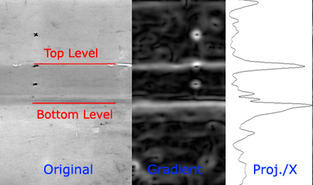 We propose to measure water levels in a basin in a sequence of images water-level.tif. We make the assumptions that the level of water is horizontal and that the
basin is never completely full or never empty.
The method is based on the detection of two maxima in the projection of the image gradient.
We propose to measure water levels in a basin in a sequence of images water-level.tif. We make the assumptions that the level of water is horizontal and that the
basin is never completely full or never empty.
The method is based on the detection of two maxima in the projection of the image gradient.
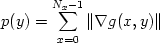
6.1 Compute the projection over the Y axis
Write the method computeXProjectionGradient which computes the intensity projection of the gradient image in the X direction.
The routines of previous sections may be used and a provided method DisplayTools.plot(double p[], String labelAbscissa, String labelOrdinate); may be used to
plot a function.
6.2 Detection of the first horizontal line
Write the routine measureLevel() which finds the ymax position corresponding to the maximum of the projection for each image
of the sequence. The input of measureLevel is a sequence of images stored in an array of ImageAccess.
6.3 Detection of the two lines
Complete the routine measureLevel() to find the two y positions corresponding to the two maxima of the projection for each image of the sequence. The basin is never empty; hence, there are at least 10 pixels between the two maxima.