 |
 |
 |
 |
 |

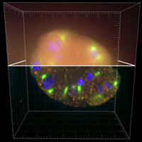
Deconvolution is one of the most common image-reconstruction tasks that arise in 3D fluorescence microscopy. The aim of this challenge is to benchmark existing deconvolution algorithms and to stimulate the community to look for novel, global and practical approaches to this problem.
The challenge will be divided into two stages: a training phase and a competition (testing) phase. It will primarily be based on realistic-looking synthetic data sets representing various sub-cellular structures. In addition it will rely on a number of common and advanced performance metrics to objectively assess the quality of the results.
Here we clarify a practical implication of the fact that our forward model relies on non-periodic boundary conditions. To illustrate our point, we rederive the standard Richardson-Lucy algorithm. The same type of modification may be required for your own algorithm if you originally developed it for circulant boundary conditions.
The Richardson-Lucy algorithm is a maximum-likelihood algorithm that is based on a Poisson noise model1. Using matrix-vector notations, we have $$ \mathbf{y} \sim \mathcal{P}(\mathbf{Ax} + \mathbf{b}) $$ where \(\mathbf{x}\) is a vector corresponding to the ground-truth image, \(\mathbf{A}\) is a matrix representing the forward operator (it is the composition of linear operators), \(\mathbf{b}\) is a constant vector representing the background signal and \(\mathbf{y}\) is a random vector modeling the measurements. The corresponding Poisson likelihood is $$ p(\mathbf{y}|\mathbf{x}) = \exp\big({-}(\mathbf{Ax} + \mathbf{b})^T\mathbf{1}\big) \times \exp\big(\log(\mathbf{Ax} + \mathbf{b})^T\mathbf{y}\big) \times \prod_{n=1}^N 1/\mathbf{y}_n!, $$ where the logarithm function is applied component-wise and \(N\) is the dimension of the measurement vector \(\mathbf{y}\).
Maximizing \(p(\mathbf{y}|\mathbf{x})\) with respect to \(\mathbf{x}\) is equivalent to maximizing the log-likelihood function $$ L(\mathbf{x}) = \log\big(p(\mathbf{y}|\mathbf{x})\big). $$ The gradient of this function is $$ \nabla L(\mathbf{x}) = \mathbf{A}^T \mathrm{diag}(\mathbf{Ax}+\mathbf{b})^{-1} \mathbf{y} - \mathbf{A}^T\mathbf{1}. $$ Imposing that this quantity vanishes leads to the following multiplicative-update algorithm: $$ \mathbf{x}_{k+1} = \mathrm{diag}(\mathbf{A}^T\mathbf{1})^{-1} \mathrm{diag}\big[\mathbf{A}^T \mathrm{diag}(\mathbf{Ax}_k+\mathbf{b})^{-1} \mathbf{y}\big] \mathbf{x}_k. $$
Usually the matrix \(\mathbf{A}\) is taken to be block-circulant and normalized such that \(\mathbf{A}^T\mathbf{1} = \mathbf{1}\);
in this case the Richardson-Lucy iteration reduces to \(\mathbf{x}_{k+1} = \mathrm{diag}\big[\mathbf{A}^T \mathrm{diag}(\mathbf{Ax}_k+\mathbf{b})^{-1} \mathbf{y}\big] \mathbf{x}_k\).
However, in the framework of this challenge the matrix \(\mathbf{A}\) has a different structure and therefore the normalization factor \(\mathrm{diag}(\mathbf{A}^T\mathbf{1})^{-1}\) is non-trivial. Note that in our reference implementation of the Richardson-Lucy algorithm (RLdeblur3D.m) this quantity is precomputed in the beginning. Please also refer to the distributed code of the challenge where the implementations of the forward operator \(\mathbf{A}\) (Direct.m) and of its adjoint \(\mathbf{A}^T\) (Adjoint.m) are made available.
The registered participants will receive soon a personalized upload link.
January 6, 2014The evaluation stage of the second edition of the challenge has started.
November 6, 2013The official stage of the challenge will last around 2 months.
November/December, 2013The training stage of the second edition of the challenge has started. Follow this link to register and receive e-mail updates.
July 17, 2013