We demonstrate the use of the WSPM toolbox through a case study. For that purpose, we use the 'single subject epoch auditory' data of G. Rees and K. Friston, which can be downloaded. These data were acquired on a 2T Siemens Magneton, 7s repetition time, 64x64x64 volumes with voxels of physical size 3mm x 3mm x 3mm. The block length was 6 volumes (42s) where the condition alternates between rest and auditory stimulation (bi-syllabic words presented binaurally at a rate of 60 per minute). The total number of volumes was 96, but the first 12 volumes are advised to discard due to T1 effects. This leaves us with 84 volumes or equivalently 14 cycles of 12 volumes.

In what follows, we assume that the current directory is where the data is located. Before we can use the toolbox, we need to do a complete standard SPM analysis since we need at least one t-contrast to be available. Here, we perform a basic analysis only (realignment, smoothing, GLM).

(1) Standard SPM analysis

• Start SPM
  >> spm fmri
  The SPM window appears.
  
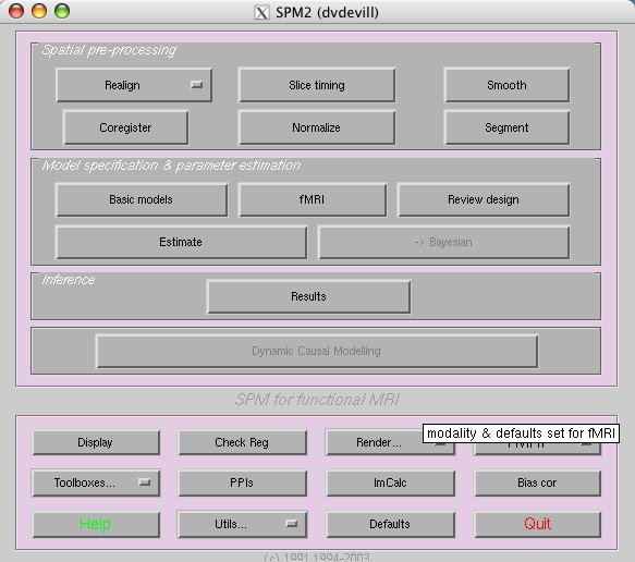
• Realign
  Select the 'realign' option from the 'Spatial pre-processing' menu
  Num subjects: 1
  Num sessions subj 1: 1
  Select volumes fM00223_016 to fM00223_099 (84 in total)
  Select: Coregister and reslice
  Select: All images and mean image
  SPM creates now the realigned volume rfM00223_016 to rfM00223_099
• Smooth
  smoothing {FWHM in mm}: 6
  Select volumes rfM00223_016 to rfM00223_99 (84 in total again)
  SPM creates now the smoothed volume srfM00223_016 to srfM00223_099
• Model setup
  Select the 'fMRI' option from the 'Model specification & parameter estimation' menu
  Select: 'design'
  Interscan interval {secs}: 7
  Scans per session: 84
  Specify design in: 'scans'
  Hemodynamic basis functions: 'hrf'
  Model interactions {Volterra}: 'no'
  Number of conditions/trials: 1
  Name for condition/trial 1: 'auditory'
  Vector of onsets - trial 1: 6:12:84
  Duration[s] (events=0): 6
  Parametric modulation: 'none'
  Other regressors: 0
• Data setup
  Select the 'fMRI' option from the 'Model specification & parameter estimation' menu
  Select: 'data'
  Select the 'SPM.mat' file
  Select the volumes srfM00223_016 to srfM00223_099 (84 in total)
  Remove global effects: 'scale'
  High-pass filter (sec): 168
  Correct for serial correlation: 'AR(1)'
• Estimate
  Select the 'Estimate' option from the 'Model specification & parameter estimation' menu
  Select the 'SPM.mat' file
• Create a t-contrast
  Select the 'Results' option from the 'Inference' menu
  Select the 'define new contrast' option from the 'contrast menu
  Name: 'T'
  Type: 't-contrast'
  Contrast: 1 0
  
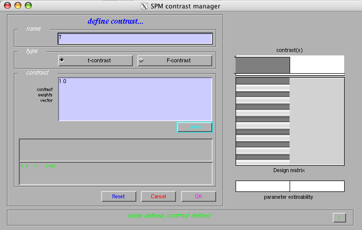
  Select 'OK' and pick the newly defined contrast in the contrast menu
  Mask with other contrast(s): 'no'
  Title for comparison: 'activation'
  P value adjustment to control: 'FWE'
  P value (family-wise error): 0.05
  & extend threshold {voxels}: 0
  SPM displays the results
  
  

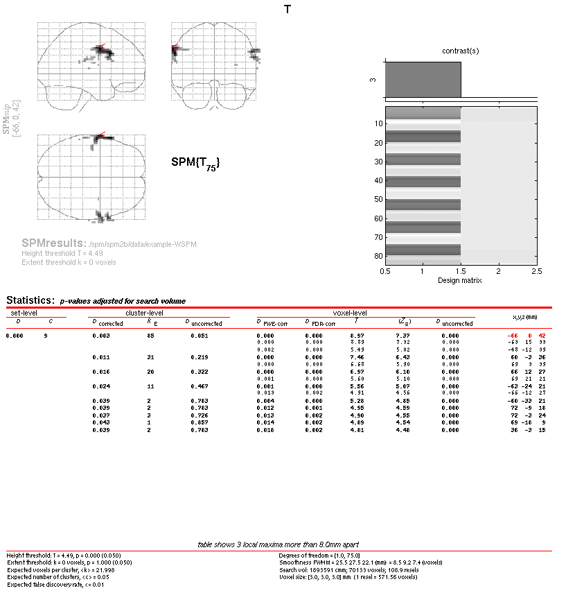
Next, we can use the WSPM toolbox to obtain results using the spatio-wavelet framework for one of the t-contrasts available.

(2) WSPM analysis

• Prepare data for a desired wavelet transform
  Select the 'WSPM' option from the 'Toolboxes' submenu
  Select the 'SPM.mat' file
  Select: 'estimate'
  Select the volumes rfM00223_016 to rfM00223_099 (84 in total), so the non-smoothed ones!
  Subsampling scheme: 'dyadic'
  Transform type: '2D+Z'
  Redundancy: 'Multiple'
  Wavelet flavor: '*ortho'
  Degree (XY-plane): 1
  Number of iterations: 1
  The toolbox computes the wavelet transform of all the volumes. There will also change the structure SPM in the 'SPM.mat' file; i.e., a substructure SPM.Wavelet is extended. You can compute as many transforms as you want.
• Generate results
  Select the 'WSPM' option from the 'Toolboxes' submenu
  Select the 'SPM.mat' file
  Select the wavelet transform; automatically if only one available (in our example: zm*ortho,1/0,1)
  Select the contrast; automatically if only one available (in our example: {T}: activation)
  P value (significance level): 0.05
  The toolbox computes the results according to the spatio-wavelet framework and adds a traditional SPM contrast to the SPM structure.
• Display results
  Select the 'Results' option from the 'Inference' menu
  Select the newly added contrast
  
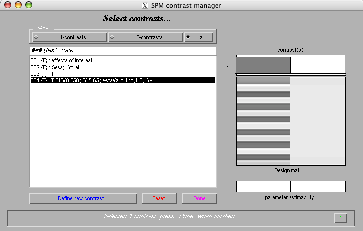
  Mask with other contrast(s): 'no'
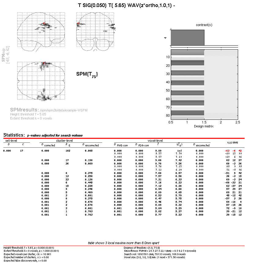
  Title for comparison: 'T SIG(0.050) T( 5.65) WAV(zm*ortho,1.0,1)'
  P value adjustment to control: 'none'
  Threshold {T or p value}: 5.65; you need to put the value that is available in the contrast title as T(XXX)
  & extent threshold {voxels}: 0
  SPM displays the results
  
  

Naming convention for the wavelet transform:

• Transform type: 'z' (2D+Z) or '' (3D)
• Redundancy: '' (none) or 'm' (multiple)
• Subsampling scheme: '' (dyadic) or 'q' (quincunx)
• Flavor:
  • B-spline flavors (for dyadic subsampling):
    '*ortho' (symmetric orthogonal B-spline)
    '*bspline' (symmetric B-spline)
    '*dual' (symmetric dual B-spline)
    '+ortho' (causal orthogonal B-spline)
    '+bspline' (causal B-spline)
    '+dual' (causal dual B-spline)
  • Polyharmonic and McClellan flavors (for quincunx subsampling):
    'Portho' (orthogonal polyharmonic)
    'Pbspline' (Rabut polyharmonic B-spline)
    'Pdual' (Rabut polyharmonic dual B-spline)
    'PBspline' (isotropic polyharmonic B-spline)
    'PDual' (isotropic polyharmonic dual B-spline)
    'ortho' (McClellan orthogonal)
    'bspline' (McClellan B-spline like)
    'dual' (McClellan dual B-spline like)
• Separator ','
• Degree in the XY-plane
• Separator '/'
• Degree in the Z-plane (if not applicable: 0)
• Separator ','
• Number of iterations

Naming convention for the contrasts:

• Original SPM contrast name
• SIG(XXX), where XXX is the significance level
• T(XXX), where XXX is the threshold to put
• WAV(XXX), where XXX is the wavelet transform name