PSF Generator

An ImageJ plugin to generate 3D microscope Point-Spread Function (PSF)

Written by Hagai Kirshner and Daniel Sage, Biomedical Imaging Group at EPFL.

Outline

PSF Generator is a software package that allows one to generate and visualize various 3D models of a microscope PSF [1]. The current version has five different models: the Gaussian model, the simulated Defocus, the scalar-based diffraction model Born & Wolf [5, 6], the scalar-based diffraction model with 3 layers Gibson & Lanni [7], and the vectorial-based model Richards & Wolf [8, 9]. In addition, we have added the Variable Refractive Index Gibson & Lanni model [10]. This model was developpent and implemented by Sameer Hiware, Indian Institute of Technology (IIT) of Bombay, Mumbia, India.

The models differ one from the other by the accuracy they introduce, while the trade-off is the required computational complexity and run-time. The plugin requires only few parameters which are readily-available for microscopy practitioners.

PSF Generator is an ImageJ plugin. Our Java implementation achieves fast execution times, as it is based on multi-threading the computational tasks and on a numerical method that adapts to the oscillatory nature of the required integrands. Potential applications are 3D deconvolution [2], 3D particle localization and tracking [3], and extended depth of field estimation [4] to name a few.

Reference

[ 1] H. Kirshner, F. Aguet, D. Sage, M. Unser, "3-D PSF Fitting for Fluorescence Microscopy: Implementation and Localization Application," Journal of Microscopy, vol. 249, no. 1, pp. 13-25, January 2013.

[10] S. Hiware, P. Porwal, R. Velmurugan and S. Chaudhuri, "Modeling of PSF for refractive index variation in fluorescence microscopy," IEEE International Conference on Image Processing (ICIP 2011) 2011, pp. 2037Ð2040.

Software

ImageJ Pre-requirement

The software provided here is a plugin for ImageJ, a general purpose image-processing and image-analysis package. ImageJ has a public domain license; it runs on several platforms: Unix, Linux, Windows, and Mac OSX. It doesn't take more than a couple of minutes to install.

Download and install

Download PSF_Generator.jar, the ImageJ's plugin. The current version is dated 19.03.2013. The plugin consist in one single JAR file; place it into the "plugins" folder of ImageJ. Do not unzip the JAR file.

Instructions

Start ImageJ and launch the plugin PSF_Generator.
Select the model using the tab and set the optics parameters. The parameters for each model are explained below.
Set the output parameters. NX, NY, and NZ are the dimensions of the output stack.
Click on the button "Generate PSF"
After a while, the stack is showed

Conditions of use

You are free to use this software for research purposes, but you should not redistribute it without our consent.
In addition, we expect you to include adequate citations and acknowledgments whenever you present or publish results that are based on it.

Richards & Wolf PSF model

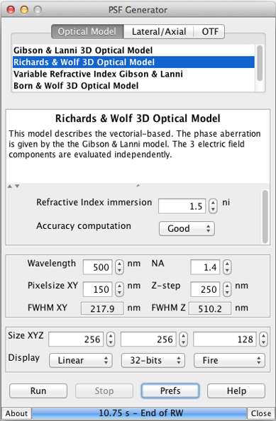
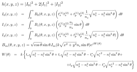
This model describes the vectorial-based diffraction that occurs in the microscope [8, 9]. The phase aberration W(Θ) is given by the Gibson and Lanni model, but the three electric field components are evaluated independently. The PSF of this model is shift invariant in the lateral directions only. This model is defined by the following equation:

Screenshot of the GUI	Spatial section XY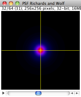	Axial section YZ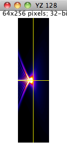
	Running time: 12.53 ms to generate a 256x256x64 stack.

Gibson & Lanni PSF model

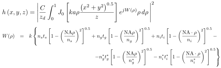
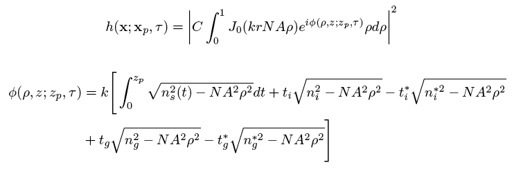
This model describes the scalar-based diffraction that occurs in the microscope [7]. It accounts for the immersion, the cover-slip and the sample layers. The PSF of this model is shift invariant in the lateral directions only. This model is defined by the following equation:

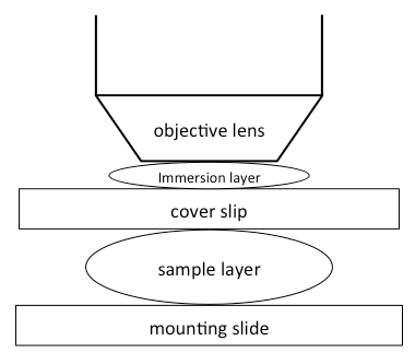
Parameter	Description
NA	Numerical Aperture of the objective lens. This value is given by NA = ni sin(Θ) where Θ is one half of the angular aperture of the lens.
n_s	Refractive index of the sample layer.
t_s	Axial location of the point source within the sample layer. The corresponding input field in the plugin is "z".
n_g	Actual value of the refractive index of the coverslip. This value is assumed to be equal to n_g* and it is therefore not used by the plugin.
n_g*	Nominal value of the refractive index of the coverslip. This value is assumed to be equal to n_g and it is therefore not used by the plugin.
n_i	Actual value of the refractive index of the immersion layer (the paper by Gibson and Lanni uses the notations n_oil).
n_i*	Nominal value of the refractive index of the immersion layer (the paper by Gibson and Lanni paper uses the notations n_oil*. This value is assumed to be equal to n_i and it is therefore not used by the plugin.
t_g	Actual value of the coverslip thickness. This value is assumed to be equal to t_g* and it is therefore not used by the plugin.
t_g*	Nominal value of the coverslip thickness. This value is assumed to be equal to t_g and it is therefore not used by the plugin.
t_i	Actual working distance between the objective and the coverslip (the Gibson and Lanni paper uses the notation t_oil).
t_i*	Nominal working distance between the objective lens and the coverslip (the Gibson and Lanni paper uses the notation t_oil). This value is given by t_i = t_i + Δ where Δ is the stage displacement. When generating a z-stack, stage displacement values are determined by the "Axial resolution" and by the "slices" input parameters of the plugin. If the number of slices is odd, then the middle slice corresponds to Δ = 0.
λ	Wavelength of the light emitted by the point source.
k	Wavenumber in vacuum of the emitted light, k = 2Π/λ.
xd, yd	Lateral position for evaluating the PSF at the detector plane. The sampling points are {x_d,n, y_d,m} = {nΔ, mΔ}_n,m where Δ is the value of the "Pixel size in object space" input parameter, n = - (N-1)/2 ... (N-1)/2 and m = - (M-1)/2 ... (M-1)/2. N and M are the "width" and the "height" input parameters, respectively of the plugin. If N and M are odd, then the middle pixel is (0,0).
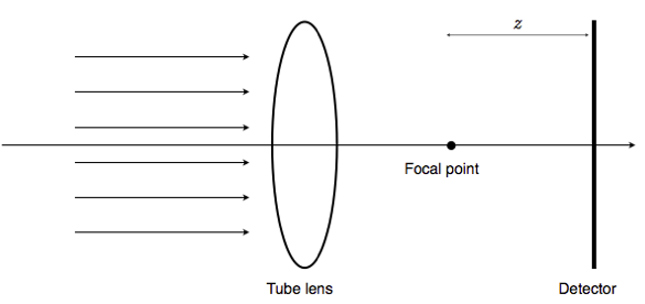
z_d	Axial distance between the detector and the tube lens. This value is assumed to be equal to the focal length of the tube lens, and for this reason the plugin substitutes NA = a/z_d in h(x, y, z).
W	The Gibson and Lanni phase aberration.
C	A normalizing constant. The value C/z_d that appear in h(x, y, z) is determined by the "normalization" input parameter of the plugin.

Screenshot of the GUI	Spatial section XY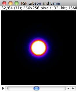	Axial section YZ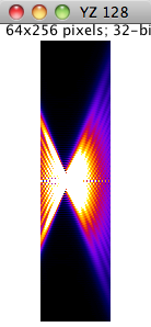
	Running time: 3.92 s to generate a 256x256x64 stack.

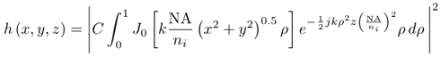
Variable Refrative Index Gibson & Lanni PSF model

This model is an extension to the Gibson and Lanni model, that describes the scalar-based diffraction that occurs in the microscope [10]. It captures the aberration that caused due to variation of refractive index within the thick specimen. This model captures shift varying nature of PSF in axial direction only by three predefined functions: linear Logarithmic, and Exponential. This model defined by the following equations:

where:

x = (x, y, z) denotes the coordinate of a point in the image plane.
x_p = (x_p; y_p; z_p) is the coordinate of the point source.
τ = (NA; n; t) is the parameter set of the imaging system in which n is the refractive index and t is the thickness.
r² = (x - x_p)² + (y - y_p)² is the point at which ray intersects the exit pupil.
J₀ is the Bessel function of first kind of order zero.

Parameter	Description
NA	Numerical Aperture of the objective lens. This value is given by NA = ni sin(Θ) where Θ is one half of the angular aperture of the lens.
n_s	Refractive index of the sample layer.
t_s	Axial location of the point source within the sample layer. The corresponding input field in the plugin is "z".
n_g	Actual value of the refractive index of the coverslip. This value is assumed to be equal to n_g* and it is therefore not used by the plugin.
n_g*	Nominal value of the refractive index of the coverslip. This value is assumed to be equal to n_g and it is therefore not used by the plugin.
n_i	Actual value of the refractive index of the immersion layer (the paper by Gibson and Lanni uses the notations n_oil).
n_i*	Nominal value of the refractive index of the immersion layer (the paper by Gibson and Lanni paper uses the notations n_oil*. This value is assumed to be equal to n_i and it is therefore not used by the plugin.
t_g	Actual value of the coverslip thickness. This value is assumed to be equal to t_g* and it is therefore not used by the plugin.
t_g*	Nominal value of the coverslip thickness. This value is assumed to be equal to t_g and it is therefore not used by the plugin.
t_i	Actual working distance between the objective and the coverslip (the Gibson and Lanni paper uses the notation t_oil).
t_i*	Nominal working distance between the objective lens and the coverslip (the Gibson and Lanni paper uses the notation t_oil). This value is given by t_i = t_i + Δ where Δ is the stage displacement. When generating a z-stack, stage displacement values are determined by the "Axial resolution" and by the "slices" input parameters of the plugin. If the number of slices is odd, then the middle slice corresponds to Δ = 0.
λ	Wavelength of the light emitted by the point source.
k	Wavenumber in vacuum of the emitted light, k = 2Π/λ.
xd, yd	Lateral position for evaluating the PSF at the detector plane. The sampling points are {x_d,n, y_d,m} = {nΔ, mΔ}_n,m where Δ is the value of the "Pixel size in object space" input parameter, n = - (N-1)/2 ... (N-1)/2 and m = - (M-1)/2 ... (M-1)/2. N and M are the "width" and the "height" input parameters, respectively of the plugin. If N and M are odd, then the middle pixel is (0,0).
z_d	Axial distance between the detector and the tube lens. This value is assumed to be equal to the focal length of the tube lens, and for this reason the plugin substitutes NA = a/z_d in h(x, y, z).
W	The Gibson and Lanni phase aberration.
C	A normalizing constant. The value C/z_d that appear in h(x, y, z) is determined by the "normalization" input parameter of the plugin.

Screenshot of the GUI	Spatial section XY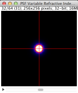	Axial section YZ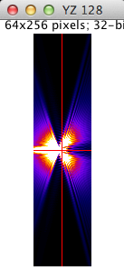
	Running time: 3.92 s to generate a 256x256x64 stack.

Born & Wolf PSF model

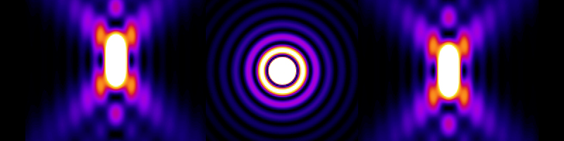
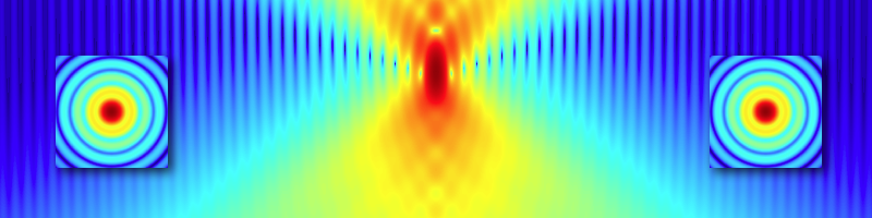
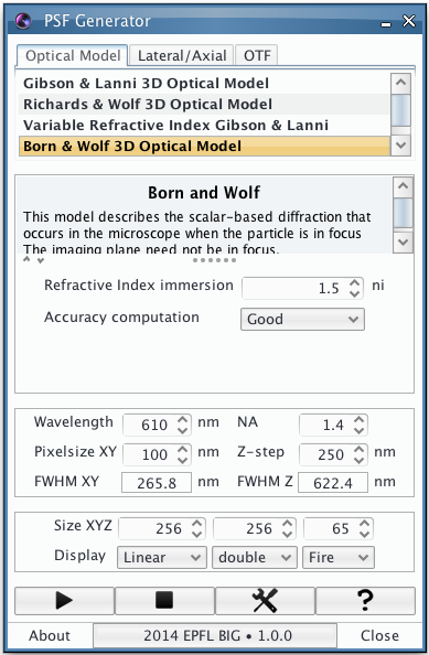
This model describes the scalar-based diffraction that occurs in the microscope when the particle is in focus [5, 6]. The imaging plane, however, need not be in focus. The PSF of this model is shift invariant in all directions. This model is defined by the following equation:

Screenshot of the GUI	Spatial section XY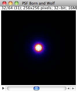	Axial section YZ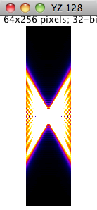
	Running time: 942 ms to generate a 256x256x64 stack.

Simulated defocus PSF model

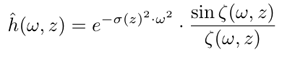
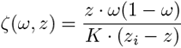
This models simulates defocusing in the Fourier domain by a modulated Gaussian function. The variance of Gaussian (σ) changes linearly with the axial axis. ω is the radial frequency which is defined by: ω² = ω_x² + ω_y². This model is defined by the following equation:

where

Screenshot of the GUI	Spatial section XY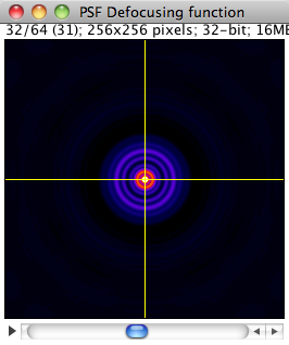	Axial section YZ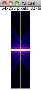
	Running time: 2300 ms to generate a 256x256x64 stack.

Gaussian PSF model

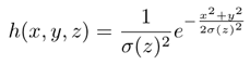
This model simulates the blurring effect with a 2D gaussian function. The variance of Gaussian (σ) changes linearly with the axial axis. This model is defined by the following equation:

Screenshot of the GUI	Spatial section XY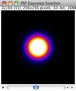	Axial section YZ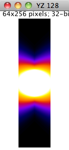
	Running time: 1800 ms to generate a 256x256x64 stack.

Bibliography

[1] H. Kirshner, D. Sage, M. Unser, "3D PSF Models for Fluorescence Microscopy in ImageJ," Proceedings of the Twelfth International Conference on Methods and Applications of Fluorescence Spectroscopy, Imaging and Probes (MAF'11), Strasbourg, France, September 11-14, 2011, pp. 154.
[2] A. Griffa, N. Garin, D. Sage, "Comparison of Deconvolution Software in 3D Microscopy: A User Point of View—Part 1," G.I.T. Imaging & Microscopy, vol. 12, no. 1, pp. 43-45, March 2010.
[3] D. Sage, F.R. Neumann, F. Hediger, S.M. Gasser, M. Unser, "Automatic Tracking of Individual Fluorescence Particles: Application to the Study of Chromosome Dynamics," IEEE Transactions on Image Processing, vol. 14, no. 9, pp. 1372-1383, September 2005.
[4] F. Aguet, D. Van De Ville, M. Unser, "Model-Based 2.5-D Deconvolution for Extended Depth of Field in Brightfield Microscopy," IEEE Transactions on Image Processing, vol. 17, no. 7, pp. 1144-1153, July 2008.
[5] M. Born and E. Wolf, Principles of Optics, 7th edition, Cambridge University Press, 2003, Chapter 8.5, pages 436-445.
[6] S. Frisken-Gibson and F. Lanni, Diffraction by a circular aperture as a model for three-dimensional optical microscopy, JOSA A, Vol. 6, No. 9, September 1989.
[7] S. Frisken-Gibson and F. Lanni,Experimental test of an analytical model of aberration in an oil-immersion objective lens used in three-dimensional light microscopy, JOSA A, Vol. 9, No. 1, January 1992.
[8] B. Richards and E. Wolf, ÒElectromagnetic diffraction in optical systems. II. structure of the image field in an aplanatic system," Proc. R. Soc. London A, vol. 253, no. 1274, 1959.
[9] F. Aguet, "Super-Resolution Fluorescence Microscopy Based on Physical Models," Swiss Federal Institute of Technology Lausanne, EPFL Thesis no. 4418 (2009), 209 p., May 28, 2009.
[10] S. Hiware, P. Porwal, R. Velmurugan and S. Chaudhuri, "Modeling of PSF for refractive index variation in fluorescence microscopy," IEEE International Conference on Image Processing (ICIP 2011) 2011, pp. 2037Ð2040.