News Overview Registration Downloads Uploads Documentation Contact Feedback Previous Edition

FORWARD MODEL

General description

The central part of the forward model is a discrete convolution of the form

$$(f*h)[\boldsymbol{n}] = \sum_{\boldsymbol{k} \in \ \mathbb{Z}^3} f[\boldsymbol{k}] \, h[\boldsymbol{n} - \boldsymbol{k}],$$ where $f$ represents the ground-truth distribution of fluorophores and $h$ represents the point-spread function (PSF).

Unlike standard formulations of deconvolution, we do not use periodic boundary conditions. Instead we will exploit the following facts.

1. The support of $f$ along the axial dimension (Z) is finite. This should be clear from a physical standpoint, since biological samples are typically very thin.
2. The support of $h$ along the lateral dimensions (X and Y) can be considered finite. This is slightly counter-intuitive, considering that the intensity of the PSF decays slowly as one moves away from the optical center (we refer to the typical hourglass shape depicted in Fig. 1). However it is a valid approximation since the object $f$ has finite support along the Z axis (thus we only need to consider a finite part of the PSF along the Z axis).

Thanks to these assumptions the convolution reduces to a finite sum. In the following subsections we discuss details of the implementation from a mathematical standpoint.

The complete forward model is given by $$g[\boldsymbol{n}] \sim Q\bigg(\mathcal{P}\Big((A\{f\})[\boldsymbol{n}] + b\Big) + w[\boldsymbol{n}]\bigg).$$ Here, $A$ is a linear operator which includes the convolution operation, the constant $b$ corresponds to a background signal, and the notation $\mathcal{P}(\lambda)$ represents a Poisson random variable of intensity $\lambda$. The latter models shot noise, which is due to the quantum nature of light. The symbols $w[\boldsymbol{n}] \sim \mathcal{N}(0, \sigma^2)$ denote IID Gaussian random variables corresponding to detector noise. Finally $Q$ is a quantization operator defined by $$Q(x) = \begin{cases} \arg\min_{n \in \mathbb{N}} |x - n| & \text{if } x > 0, \\ 0 & \text{otherwise} \end{cases}$$ and $g$ represents the measured data. Note that our model is based on the simplifying assumption of a photon-counting detector. Thus it does not involve a gain parameter and the measurements $g[\boldsymbol{n}]$ can directly be interpreted in terms of photons.

Forward Operator - Implementation

The convolution product $h*f$ can be represented in matrix form as $\mathbf{Hf}$, where the vector $\mathbf{f}$ contains the samples $f[\boldsymbol{n}]$ in lexicographic order and $\mathbf{H}$ is a block-circulant matrix constructed from the samples $h[\boldsymbol{n}]$. This is also one of the most common deconvolution settings used in the literature.

Despite the popularity of using a circulant operator in the deconvolution setting, such a choice implies periodic boundary conditions for the object of interest. This particular assumption is quite unrealistic and, for real data, often leads to severe artefacts in the reconstuction. In this challenge, we provide a forward model that serves as a better approximation of the process taking place in the microscope. Instead of assuming specific boundary conditions, we explicitly state our lack of information outside the boundary of the image. Mathematically speaking, the employed forward operator, $\mathbf{A}$, can be described as the composition of the following operations:

$$\mathbf{A}\mathbf{f}=(\mathbf{M}\mathbf{H}\mathbf{Z})\mathbf{f}.$$ where $\mathbf{H}$ is a circulant convolution matrix that admits a fast FFT implementation and $\mathbf{M}$ and $\mathbf{Z}$ are suitable masking operators. Specifically, $\mathbf{M}$ is a masking operator which returns only the part of the circulant convolution that is valid. This means that the operator $\mathbf{M}$ truncates those parts of the linear convolution which are computed based on the periodic boundary assumption. In particular, for an object $f$ of size $[N_x,\, N_y,\, N_z]$ and a PSF $h$ of size $[L_x,\, L_y,\, L_z]$, the size of the valid part of the linear convolution is equal to $[N_x-L_x+1,\, N_y-L_y+1,\, N_z-L_z+1]$. This is always true if we assume that the support of $f$ is larger than that of $h$ in all dimensions.

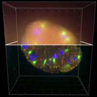
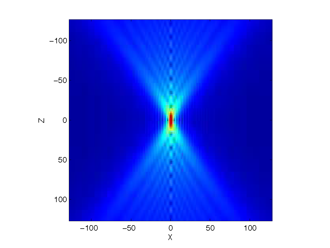
As it was mentioned above, biological samples are typically thin while the effect of the PSF on the measurements is larger in the axial direction than in the lateral one (see Fig. 1). Thus, it is reasonable to use a PSF whose support in the axial direction is broader than the support of the object at the same direction. These two facts combined suggest that the convolution in the Z-dimension must be performed so that the roles of the object and the PSF are interchanged. Therefore, for an object $f$ of size $[N_x,\, N_y,\, N_z]$ and a PSF $h$ of size $[L_x,\, L_y,\, L_z]$ where $L_z > N_z$, the forward operation, $\mathbf{A}\mathbf{f}$, results to a measured object of size $[N_x-L_x+1,\, N_y-L_y+1,\, L_z-N_z+1]$. This outcome is achieved by using the linear operator $\mathbf{Z}$, which zeropads the object $f$ in the axial direction so that its size becomes equal to $2L_z-N_z$. For more details, we refer the participants to the documentation of the Matlab scripts as well as to the distributed code of the challenge where computationally efficient implementations of the forward operator $\mathbf{A}$ (Direct.m) and of its adjoint $\mathbf{A}^T$ (Adjoint.m) are made available.

---

^{[1]. H. Kirshner, F. Aguet, D. Sage, and M. Unser. 3-D PSF fitting for fluorescence microscopy: implementation and localization application. Journal of Microscopy, 249(1):13-25, 2013.↩}

^{[2]. S. F. Gibson and F. Lanni. Experimental test of an analytical model of aberration in an oil-immersion objective lens used in three-dimensional light microscopy. Journal of the Optical Society of America A, 9(1):154-166, 1992.↩}

Important Dates